The proportional hazards model has been used in maintenance optimization since the 1990’s to combine age data and condition monitoring data to more accurately represent the equipment health condition (Jardine, Lin, and Banjevic 2006). While a condition-based maintenance approach based on the proportional hazards model has previously been used to determine optimal replacement policies for systems consisting of a single unit or component, it is only recently that an analogous method for multi-component systems has been developed (Tian and Liao 2011). This section presents the structure of a representative existing multi-component reliability model and identifies some shortcomings of that model. An extended equipment reliability model, that makes use of the proportional hazard model, is then proposed and discussed.
A generalized reliability model describing an older model of a rotating turret fitted with a 40mm gun is described in this section.
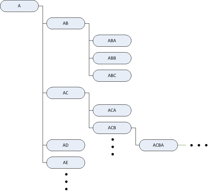
The gun & turret reliability model is described in a tree structure, similar to that in Figure 2.4. The root of the tree is the complete system, including the complete gun, turret, etc. The system is then broken down hierarchically into smaller and smaller sub-systems. In the case of Figure 2.4, the root node labeled “A” would be the complete gun and turret, “AB” could be the gun system, “ABA” the barrel, “ABB” the magazine, and so on. Each leaf node in the tree constitutes a characteristic component, for example a fastening bolt in the mechanism. There may be more than one bolt of the same type, so a leaf may describe multiple items. The same kind of bolt may also be used elsewhere on the system, but would then provide a different function, with different load and usage characteristics, and is thus described by a different leaf in the tree. The 40mm gun & turret model consists of roughly 1000 characteristic components, describing around twice as many items in a tree more than seven levels deep.
Some components of the system are infeasible to maintain at the location of the system. One example is components that are integrated together into an electronics-box or similar. Such collections of components are grouped together as replacement units, which are expected to be replaced and/or maintained as a single component. Replacement units are described by non-leaf nodes in the tree structure, for example node “ACB” in Figure 2.4 could be a replacement unit encapsulating all components listed as children of that node. This aggregation describes structural dependence between some of the components, as performing maintenance of one involves maintenance of the entire replacement unit. While all replacement units are described by non-leaf nodes, all non-leaf nodes do not constitute replacement units.
Each leaf and replacement unit node in the model describes a number of characteristics of the component which it represents. Available information for each component includes:
The existing reliability models, as outlined in Section 2.2.1, have some general limitations worth addressing. Firstly, the current models adequately describe structural dependence between the different components in the model, but they do not include information about economic or stochastic dependence. If equipment is being made unavailable for maintenance, it is reasonable to assume that there are economic benefits to performing multiple maintenance actions at the same time. If enough staff is available, it is possible some maintenance actions can be performed simultaneously. Even if each maintenance action is done sequentially, actions such as transporting the equipment to and from the maintenance facility creates opportunities for reducing downtime and costs. Stochastic dependency is likely present as well, but is harder to quantify and generalize as it is highly dependent on the specific structure of each type of equipment.
A second deficiency of the existing model is that it only includes aleatory uncertainty. The distribution for expected lifetime and failure intensity for each component is used during initial system manufacturing, to determine the probable set of spares required to keep the system functional for a predetermined period of time. Epistemic uncertainty may in this scenario be addressed to some extent by assuming a worse, or worst-case, failure intensity, but if that is the case, the underlying epistemic uncertainty considerations are not included as a part of the existing reliability model.
Finally, the current reliability model does not account for the effect of covariates on the expected failure rate of the different components. Covariates are explanatory variables, modeling how different parameters affect the hazard rate of each component. This is a logical omission when considering that the existing model was designed for resource allocation, under the assumption of a fixed usage-profile, for a determined period of time. Over that period, and under the fixed usage-profile, any effect of covariates will be constant and can thus be incorporated as part of the assumed lifetime distribution. However, when seeking to determine system status given an historic usage profile, and estimating future maintenance needs given a planned usage profile, covariates allows known and planned circumstances to be included in the reliability calculations.
Three rectifiable shortcomings of the existing reliability model have been identified when it comes to tactical level maintenance planning. Economic dependence is not addressed, epistemic uncertainty is not explicitly accounted for, and the effect of covariates on equipment reliability is not included.
This section proposes a reliability model, which is based on the reliability model structure described in Section 2.2.1, and addresses the shortcomings identified in Section 2.2.2. It consists of a refined model structure, and contains new model components describing maintenance events, failure rate and the effect of covariates.
An overview of the proposed model structure is presented in Figure 2.5. In order to be able to incorporate usage information in the model, a unique model instance will be created for each piece of equipment being maintained. The model then consists of two main components; a list of component types which is shared among all model instances, and a list of components which is unique for each instance. One key difference from the model described in Section 2.2.1 is the use of a flat component list, rather than a tree structure. The structural dependencies are thus hidden from view in the proposed list structure, which is intuitive when focusing on the reliability of individual pieces of equipment, as replacement units will behave as a single component from the equipment operators point of view. A second difference is the use of component instances. Each item described by a defined component type will generate a component instance. For example, component type “ABA” in Figure 2.5 may describe a type of washer of which there are two instances per piece of equipment; “C1” and “C2”. The component type still describes component characteristics, such as lifetime distribution, cost and mean time to repair. Each component instance contains information associated with a particular item, that is, the current hazard rate.
A maintenance event occurs when maintenance is performed on a piece of equipment. The maintenance event component of the proposed equipment reliability model seeks to describe the incurred cost and the required time for a maintenance event. The simplest way of estimating the costs and time consumed, is to simply sum the cost and the mean time to repair of each of the maintained components. On top of this estimate, the proposed model adds a setup-cost and a setup-time.
The actual cost of a maintenance event is thus modeled as follows: The setup cost, C0, is added to the cost of each maintained component, CCi. This means that the total cost, Ctot, of maintaining a set of components, M, can be described using the following formula:
 | (2.1) |
The actual time consumed for a maintenance event is modeled analogously. The setup time, T0, is added to the MTTR of each maintained component, MTTRi. This means that the total time consumed, Ttot, is described using the following formula:
 | (2.2) |
In the existing equipment model, the failure rate of each component is modeled using the exponential distribution function, which assumes a failure rate that remains constant over time using a single scale parameter, θ.
 | (2.3) |
In this proposed model, each component is instead described by the Weibull distribution function, which allows the failure rate to change as a function of time. This is achieved by the introduction of a shape variable, β. In addition, both the scale and the shape variables are assigned a probability distribution, describing the confidence in the value of each parameter. Assuming a normal distribution for each, the failure rate of each component in the model is described as:
 | (2.4) |
Where λ = N and ξ = N
 .
.
Covariates are explanatory variables, modeling how different parameters
affect the hazard rate of each component. Each covariate is described as a
function of time, zi , which contains the measured entities for covariate
i.
The effect of covariates on the hazard rate of each component in the proposed equipment reliability model is described using the Cox proportional hazards model (Cox 1972). An exponential function is thus used to adjust the baseline hazard rate, generating an expression for the hazard function of each component as follows:
 | (2.5) |
where z(t)α = ∑
i=1nzi αi. The column vector α indicates the degree of influence
that each covariate has on the hazard function.
The proportional hazards model is here illustrated with a small example, initially
disregarding the epistemic uncertainty. For ease of calculation, the assumption that
the component exhibits an exponential failure distribution function is kept.
In other words; F = 1 - e-θt, from which we can derive the baseline
hazard rate. From the discussion on reliability modeling in Section 1.4 we
have:
 | (2.6) |
This gives the baseline hazard rate:
 | (2.7) |
Now lets assume there are two covariates affecting the hazard rate in this example,
and that they are described by the functions z1 and z2
 . The expression for the
hazard rate at time t then becomes:
 | (2.8) |
By assigning values to the variables, and measuring or assuming values for the
covariates, the hazard rate for the component can be calculated. For example, θ =  ,
α1 = 0.05, α2 = 0.1, z1
 = 1.0 and z2
 = 2.0 gives:
 | (2.9) |
The risk of failure at time t for the component in this example is 0.021, or 2.1%. By comparison, the baseline hazard rate, ignoring the effect of covariates, is 1.7%.
If we instead of assuming known fixed values for the parameters in the example, had estimated parameters from observational data, each parameter would be associated with a probability distribution describing the confidence in the estimated value. This is achieved by substituting the proposed formula for baseline failure rate, Equation 2.4, as well as associating each covariate weight α with a probability distribution.
For a newly developed system, without historical data, the proposed reliability model would initially be constructed from existing reliability models created during development. As data from use and maintenance actions become available the idea is to integrate that information into the model to provide the best possible estimations of equipment behavior. This section looks into how the current model can be integrated into the proposed model, and how to fit the proposed model to historical data.
The currently existing models make use of a tree structure with leaf nodes describing components, and some non-leaf nodes describing replacement units. For the purpose of the proposed model, the components included in a replacement unit do not have to be represented individually. To integrate the data from an existing models tree structure, into the proposed models list, a tree traversal algorithm has to be applied. Since the order of the components in the resulting list is not important, either a depth-first or a breadth-first approach can be used. An example using a depth-first approach is here illustrated with pseudo-code:
In the proposed model, weibull distributions are used to describe the baseline hazard rate of the different components. In the absence of historical data however, the initial failure rate distribution for each component will be the exponential distribution assumption available for each component from the existing equipment model. This is facilitated by the fact that β = 1 makes the weibull distribution identical to the exponential distribution, as can be seen in Equation 1.6. This essentially means that all components will initially be assumed to follow an exponential distribution, as in the existing equipment reliability model. When it comes to fitting the distribution parameters from collected historical data, the differences in distribution assumptions comes into play.
The process of determining distribution parameters is complicated by the fact that the reliability of the model is also affected by covariates. The distribution assumption in the existing models, as described in Section 2.2.1, integrate the effect of covariates for a baseline usage-profile.
Through collected data, observations on component lifetimes will be available over a finite time. The available observations are thus going to be censored. Right-censoring occurs when a tracked component is removed from monitoring before failure has occurred. Left-censoring occurs when a component is added to monitoring after already being in use for an unknown period of time. Indeed, a component may be both right- and left-censored, as well as passing through periods of time without monitoring. This scenario is called interval-censoring. Censoring further complicates the estimation of survival models (Fox 2002).
The freely available language for statistical computing ’R’ (R Development Core Team 2011), includes an implementation of the Cox proportional hazards model in the survival library (Therneau and Splus-¿R port by Thomas Lumley 2011). Using R, a survival model can be described and fitted to data in one step. As an illustration, the example model in Equation 2.8 included two covariates, z1 and z2, and can be represented and fitted to data per the example below:
The first argument to the ’coxph’-function consists of a survival model with the observed events mapped the observed covariates. The first two referenced columns, ’start’ and ’stop’, are used to describe when observations were made, allowing for both left- and right-censored observations to contribute to the estimation. Other referenced columns are ’failure’, which indicates whether a failure occurred at the corresponding row of observations, and ’z1’ and ’z2’ which contain the covariate values for each observation. The second parameter, ’data’, is a so called data-frame, which for the purposes of this example can be thought of as a matrix with named columns containing the observations. The column names in the data set correspond to the names supplied to the survival model given in the first parameter.
To provide an example of a model fitted to data, a simulated set of observations
was created by simulating observational data for a hypothetical component with a
hazard rate described by Equation 2.8. That is, two covariates and a baseline hazard
rate h0 =
=  . 45 applications of the hypothetical component was observed for a
duration of 1000 hours each. Covariate z1 was set to the absolute value of a normal
distributed parameter with a standard deviation of 10, z2 was set to the value of a
parameter uniformly distributed between 0 and 5. The data was generated such that
when one component would fail, a new component would take the failed components
place and thus would keep generating observational data but from a component age
of 0.
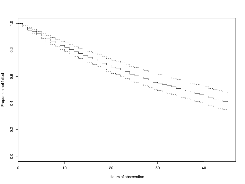
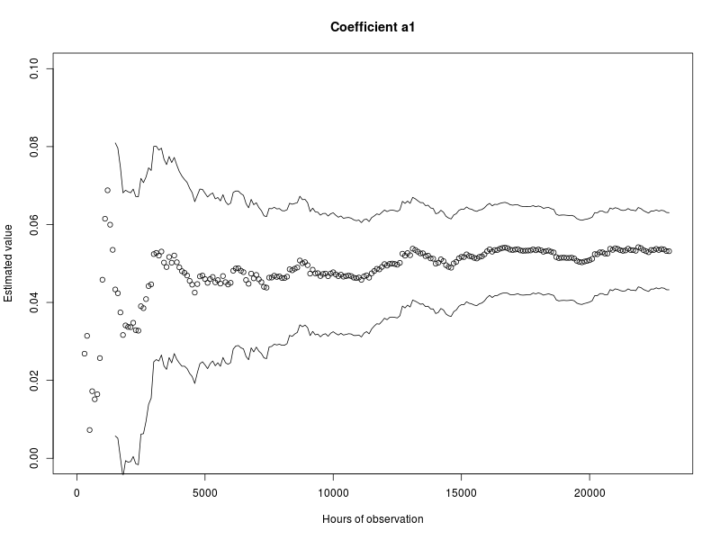
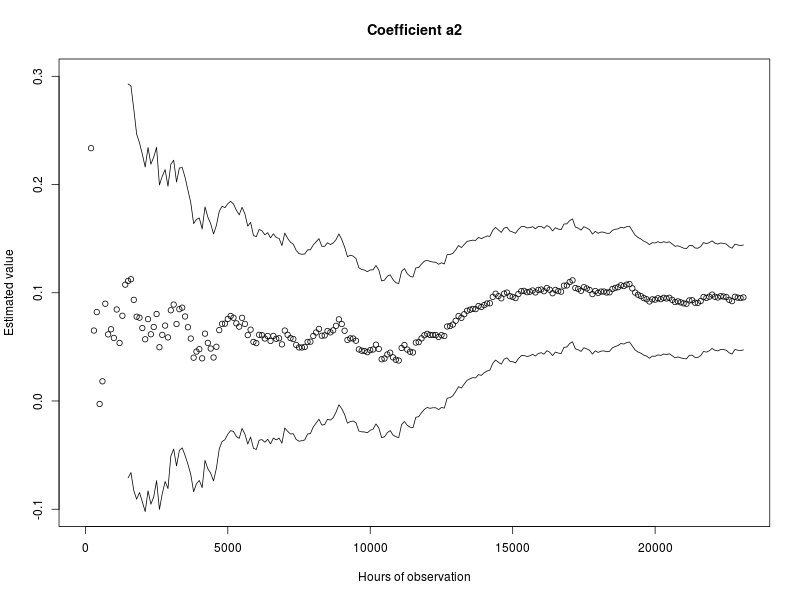
The resulting data set included 799 observed failures. The covariate weight α1 was estimated to be 0.053, with a 95%-confidence interval of 0.043 < α1 < 0.063, α2 was estimated to be 0.096, with a 95%-confidence interval of 0.047 < α2 < 0.144. The estimated failure distribution function, with the corresponding confidence interval lines, can be seen in Figure 2.6. The source code used to generate the results in this example is available in Section 3.1.

The proposed equipment reliability model described in this section was developed to address three identified shortcomings in the current models. These shortcomings were the lack of economic dependence, lack of explicit epistemic uncertainty and the omission of the effect of covariates. Each of these shortcomings are discussed in a separate subsection below.
Economic dependence between the components was added by the introduction of a setup-cost, consisting of an economic cost, C0 and a setup time-period, T0 that are required for any type of maintenance to take place. The introduction of these costs allows for the model to represent the benefits of performing multiple maintenance actions during the same maintenance occasion. Information about the initial setup-cost and setup-time depends on factors such as the distance to the nearest workshop, availability of spares and staff, etc. It is thus inconvenient to try and store these values in the equipment reliability model, but instead they are suitable to be derived from an overarching maintenance support organizational model, which is the topic of Section 2.3.
Epistemic uncertainty describes the confidence in the equipment reliability model. The structure of the system is well known as specified in design documents, including the reliability model described in Section 2.2.1, and is also verifiable by inspection. The lifetime distribution, associated failure rate and effect of covariates, that make up the proportional hazard rate model, are not so easily determined. In this proposed reliability model, epistemic uncertainty is modeled by using a distribution function to describe the parameters to the lifetime distribution functions associated with each component.
The baseline failure rate of components was extended from a simple exponential model, to a weibull model allowing epistemic uncertainty to be included in the form of probability distributions associated with the scale and shape parameters. The proportional hazards model used to describe the effect of covariates includes epistemic uncertainty by associating each covariate weight with a probability distribution.
During the life cycle of a type of equipment that is being monitored, the epistemic uncertainty is expected to change as a function of the available monitoring data. To illustrate this effect, the example from Equation 2.8 can be revisited. The estimated failure distribution function available after observing 45 applications of the example component for 1000 hours is available in Figure 2.6. The resulting estimated covariate weights with the corresponding confidence intervals were also given. To illustrate how the epistemic uncertainty changes as a function of time, the estimated value and confidence of the covariate weights α1 and α2 were plotted as a function of the total number of observed hours across all 45 applications. The resulting graphs are included in Figure 2.7 and Figure 2.8. Details of how the graphs were generated, including source code, can be found in Section 3.2.


The effect of covariates on each component in the proposed equipment reliability model is described using the Cox proportional hazards model (Cox 1972).