
The topic of this text is the creation of decision support for tactical level maintenance planning. Three required components for solving the problem were identified in Section 2.1.3; an equipment reliability mode, a maintenance support organization model and an optimization method as illustrated in Figure 2.3. An equipment reliability model that captures the information known about equipment components and units were proposed in Section 2.2. Section 2.3 proceeded to suggest an organization model that captures the structure of the maintenance support organization while integrating an interface with the equipment reliability model. The remaining required component is an optimization method that can elicit the information captured in these models in such a way to make it available to support a decision maker, which is the topic of this section.
The optimization process will operate on a set of input parameters to an implementation of the maintenance organization model. Input parameters can, for example, include maintenance policy parameters for multiple locations in the organization, as well as different permutations of resource allocations within the modeled organization. Given a set values for the input parameters, the organization model is used to determine the expected outcome in terms of availability, cost and risk.
Multicriteria decision aid includes elicitation of preferences from the decision maker, and structuring the decision process (Ehrgott 2005). It is here proposed that the elicitation of the decision makers preferences is realized through a cooperative process between the decision maker and the decision support system. By having the optimization process generate a best effort Pareto-optimal set1 of solutions, the decision maker will be able to make an informed trade off between the different criteria. This provides the decision maker with an opportunity to integrate his or hers preferences and knowledge of the problem. In addition, it is expected that the sets of solutions presented by the decision support system will prompt the decision maker to make alterations to the maintenance organization model and/or the equipment reliability models. This work flow is illustrated in Figure 2.3.
The optimization algorithm needs to be designed such that it can be used usable together with the proposed maintenance organization model. It also needs to be able to generate a set of best effort Pareto-optimal solutions. These requirements can be broken down as follows:
If an analytical expression for the optimization problem could be derived, an analytical optimization method that provably finds the Pareto-optimal set of results could be sought. In the proposed organizational model, there are many objects which will depend on each other in different ways over the simulated time of the model. There are also agents making decisions based on thresholds which can cause discontinuities in the search space. For these reasons, an analytical expression of the problem is hard to formulate, and heuristic optimization methods were sought. The most straight-forward way to derive information regarding the expected performance of the proposed organization model for a given set of input parameters is to simulate the outcomes. Simulation-based optimization thus appears as a promising approach and has been chosen for the proposed optimization method in this section.
The proposed optimization method is broken down into two parts; the first part concerns evaluation of the organizational model given a set of input parameters, and the second part concerns finding the set of input parameters which will generate the sought best effort Pareto-optimal solutions. For the first part, the availability and cost performance criteria of the proposed organizational model for a given set of parameters is considered to be stochastic variables. The estimated mean value and variance of each can thus be determined through the collection of a number of observations of the variable, where each observation is the outcome of a simulation. In other words; Monte Carlo simulation.
Simulating the proposed organizational model over a certain simulated time period, for a given set of input parameters, will generate an observed value of achieved availability, as well as an observed incurred cost. Each of these two are here considered to be independent stochastic variables. Samples of each variable can be collected through additional simulation runs.
Determination of the estimated mean value, m, and estimated variance, σ2, of a stochastic variable, X, from a number of observations, n, is straight forward. See for example Blom (1989) or any other introductory text to statistics:
 | (2.10) |
 | (2.11) |
When comparing two different stochastic variables with each other, it is also of interest to know the variance of the estimated values, i.e. the measurement error from the limited number of observations rather than the variance of the observed variable itself. From Blom (1989) we get the following expression for the variance of the estimated mean value:
 | (2.12) |
For the variance, a confidence interval at the α-level can be determined:
 | (2.13) |
The variance, ω2, in Equation 2.12 is the true variance of the observed stochastic variable. As is evident from the equation, the variance will tend towards zero with increasing numbers of samples, n. However, the true variance of the stochastic variable is not known, as Equation 2.11 is merely an estimate. To more confidently be able to compare the mean of two stochastic variables, a conservative measure of the population variance can be used. One approach is to use the following expression for the ceiling on the observed variance (Mercer 2000);
 | (2.14) |
where M is the maximum observed value and H is the harmonic mean. For the purposes in the here proposed optimization method, the ceiling of the estimated variance in Equation 2.13 is used rather than the expression for the upper bound in Equation 2.14.
Quantified epistemic uncertainty may be present in the input parameters when evaluating an instance of the proposed organizational model. Simulation runs for a fixed set of values for the input parameters will only yield information on the aleatory uncertainty inherent in the model. The epistemic uncertainty can be accounted for through randomizing the input parameters according to their quantified uncertainty before each simulation run. This technique is called “double randomization” (Marseguerra, Zio, and Podofillini 2004).
It is here proposed to use the algorithm “non-dominated search genetic algorithm” (NSGA-II) (Deb, Pratap, et al. 2002), since it has been shown to work with a combination of Monte Carlo simulation to include both epistemic and aleatory uncertainty in the optimization (Liu and Frangopol 2004; Bocchini and Frangopol 2011).
The algorithm NSGAII comprises a number of steps, illustrated in Figure 2.11. In summary, an initial population of individuals is created after which fitness is evaluated and selection performed. This is followed by a reproduction function to select individuals for reproduction through the crossover function. The resulting population is passed through a mutation function before the selection process is begun anew.
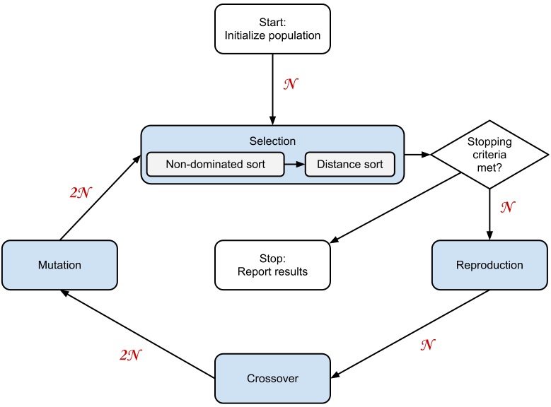
In the following, the term solution is used to refer to a specific individual in the population. Each solution is represented by a specific genome, which consists of a number of bits. The following are descriptions of the general NSGAII steps presented in Figure 2.11:
 ,
where M is the number of objectives and N the population size (Deb,
Pratap, et al. 2002).
As solutions become better and better, the size of the first front, the non-dominated set, will eventually increase and the distance sort will be used to a larger and larger extent as the optimization progresses towards a best effort Pareto-optimal set.
To be able to use NSGAII to find optimal sets of input parameters to the organization model, an interface must be designed such that the information elicited from each solution using Monte Carlo simulation can be represented as an individual in a population of solutions. Such an interface must implement a genetic representation, a fitness function and the crossover and mutation operators. Using the proposed organization model, a number of different problems can be studied depending on the choice of parametrization of the model. For readability, the discussion below uses an example parametrization throughout, that involves determination of initial allocation of a set of spares among three locations, and a set of policies for each of two of the involved locations.
The first section contains a single bit for each of the spare items that are to be part of the initial allocation. The bit not a binary number, but instead a number with the same base as there are location options to place the bit. In this example, 3. Every bit in the first section thus has a value between 0–2, representing the three different location options. If there are thirty different spares to be allocated, this first part of the genome is 30 bits long.
The second section uses five bits for each policy value of each location. In this example there are three policy values and two locations making for a total of another 30 bits added to the genome. The policy values are two integer values for “max spares level” and “reorder level”, and one float value for “preventive replacement threshold”. The integer values are stored using five binary bits. The float value however is a special case. The actual float value is stored in the last bit, i.e. bit number 44 and 59 in Figure 2.12. The first four bits are used to provide a consistent way to describe the precision of the float value when it comes to crossover and mutation operations where it will receive special handling as discussed in the corresponding sections below.
In the example problem discussed here, there are four criteria; maximization of the expected availability, minimization of the observed availability variance, minimization of the expected cost and minimization of the observed cost variance. When a genome is interpreted and a solution created through a number of Monte Carlo iterations, upper and lower bounds corresponding to a given confidence interval can be created for each of the four optimization criteria using the formulas in Equation 2.12 and Equation 2.13 respectively. There is a risk that a scenario with a low degree of confidence could by chance dominate another scenario, but that the domination relationship could change if the confidence of the solution was increased through the running of additional Monte Carlo iterations. To minimize this risk, the upper bounds for availability and cost variance are used as optimization criteria keys, instead of the actual estimated values. This will describe low confidence solutions as being associated with relatively higher risk than high confidence solutions, which is intuitive.
When the crossover point happens to be on a float value, the crossover happens as described, with the exception of the float that was at the crossover point. That particular float value is instead assigned a random value in the range described by the corresponding float value of the parents.
When embedding the Monte Carlo technique in a genetic algorithm, a technique called the “drop-by-drop” technique can be applied to reduce the computational requirements (Marseguerra, Zio, and Podofillini 2005). The technique exploits the fact that a genetic algorithm will evaluate the best chromosomes a large number of times. This allows for a reduced amount of Monte Carlo iterations to be performed when initially evaluating a solution, in effect creating a meta-model for the evaluation of a specific genome. For each iteration of the genetic algorithm, another set of Monte Carlo iterations is added to each solution, gradually refining the results of the best solutions. This means that as the search progresses, and the non-dominated set of solutions become larger, the average refinement of the model estimates increases.
Another possible way of mitigating computational requirements in this proposed optimization method is bookkeeping of calculation results from specific genomes, which will speed up calculations significantly (Okasha and Frangopol 2009). In this proposed method, results from all performed Monte Carlo iterations of each solution is kept around for as long as the solution is in the population, facilitating the “drop-by-drop” technique presented above.
This section details key components of the implementation of an example organization model matching the one used in the previous section, and illustrates from usage of the proposed optimization method on the example model. The implementation discussed here makes use of a python package implementing the NSGAII-algorithm, as well as a package detailing the model description and the interface to the genetic algorithm. The details of the implementation of each of those is available as part of Section 3.4.
The genetic representation of the parameters to each solution in the population are determined by a number of variables defining the model and its representation:
Similar to the illustration of the example model genome in Figure 2.12, for every spare there is a corresponding “bit” at the beginning of the genome. In this case, 90 bits are reserved for initial spare allocations. Maintenance policies for each type of spare for each location are then appended using the number of “bits” hinted at above; i.e. 16 bits per policy a 6 policies giving a total genome length of 90+6*16=186.
The implementation of the domination function, used by the non-dominated sort implementation in the NSGAII-package, is defined as follows:
The objective keys on which it operates are retrieved from the model interface to the genetic algorithm, and is defined as follows:
As is evident from the code, three of the objective values are inverted, which will mean that the domination function will favor smaller values over larger values.
Running the proposed optimization method, given the model and method implementations detailed in Section 3.4, is reduced to generating the initial population and a simulation loop defining the stopping criteria. In the code below, a manual stopping criteria was used. The code snippet also works as an illustration of the composition of the genome for each individual in the population.
The optimization example in the preceding code snippet is here used to illustrate some optimization results. The optimization was performed using a population size of 100 solutions, and a drop size of 6, i.e. the number of Monte Carlo simulations per generation using the drop-by-drop technique. The optimization procedure converged to produce a non-dominated set of solutions as large as the population size after 43 iterations. This is interpreted to mean that the chosen genome representation, crossover function and mutation function allows convergence towards a best-effort Pareto optimal set.
After 74 generations, the improvements in the solutions between generations was no longer obvious from a study of the plotted results. The results from the 74th generation are used for the following presentation and discussion. While better results are expected from running significantly more generations, the limited computational capacity available to the author has prompted the choice of the 74th generation, as it provides a sufficiently good solution set to serve as a representative example.
The first plot presented here, Figure 2.13, compares the achieved expected availability versus cost between the different solutions. The results form a curve-like shape, with a clear knee between costs of 1.1-1.2 million. The interpretation is that availability can be increased in proportion to costs up until around a cost of 1.1-1.2 million, where the returns in availability on additional investments are marginal. A solution at or near the knee appears to be a good trade off for a decision maker in terms of expected availability per expected cost. However, as can be seen from the color coded variance in achieved availability, solutions with high expected availability also exhibit more variance. The interpretation is that what might at first appear as a very appealing solution at the knee, has the drawback of exhibiting a relatively higher risk of deviating from the expected performance compared to solutions with lower expected cost and availability.
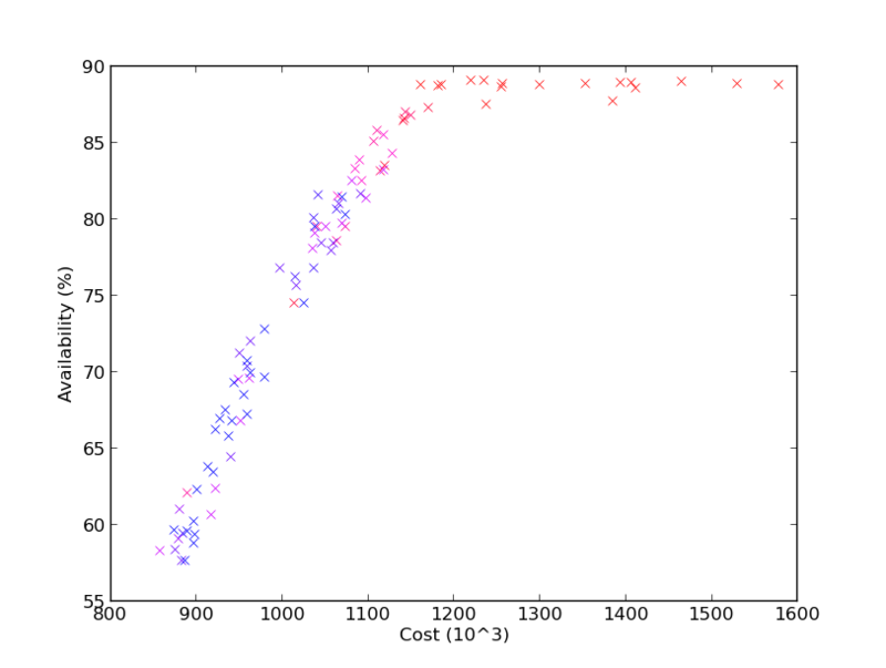
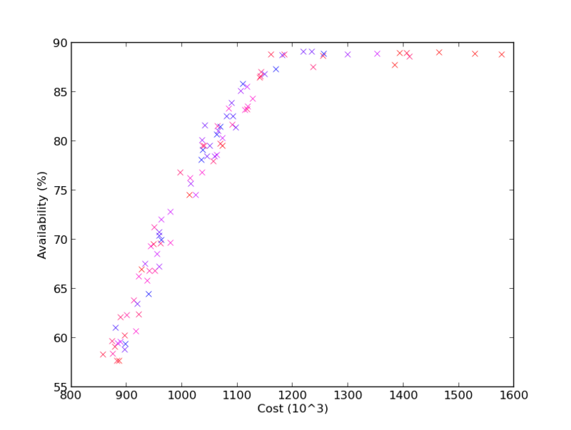
Figure 2.14 again compares achieved expected availability versus cost, but this time the color coding shows the relative variance in achieved cost performance. Solutions with high and low cost variance are interspersed throughout most of the graph, with some low variance solutions also in the higher availability range, including around the knee. The interpretation is that a solution with relatively lower cost variance can likely be picked regardless of the availability versus cost trade off made by the decision maker.
So far only relative variance values have been presented. Figure 2.16 displays achieved expected availability versus availability variance, where it is evident from the scale on the horizontal axis that the achieved availability variance in generally low. Assuming a normal distribution for achieved availability, and a variance of 0.014, a solution with an expected availability of 90.0% will achieve no less than 87.7% with 95% confidence. The interpretation is that availability variance in this simulation can be ignored, as it is sufficiently low in all found solutions.
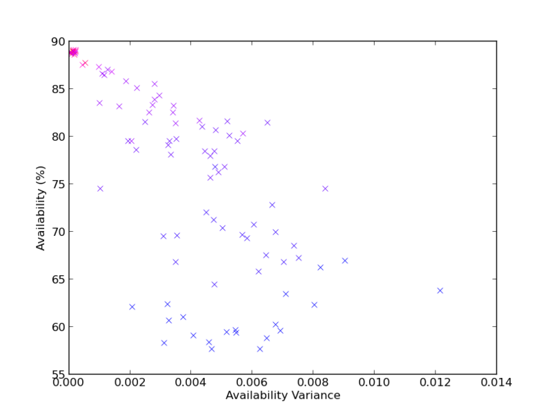
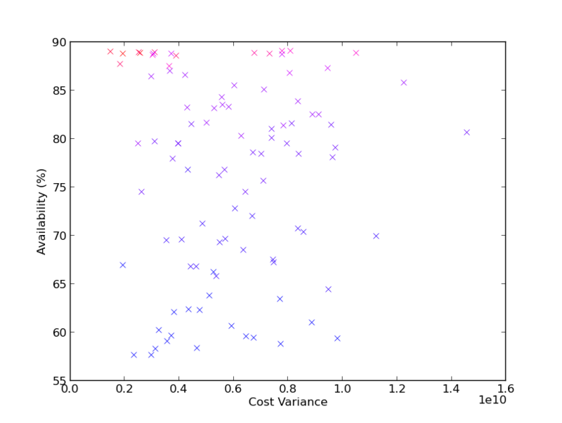
Figure 2.16 compares the expected availability versus the cost variance. Cost variance values are high. Assuming that achieved costs are normally distributed, an expected cost of 1.1 million, with a variance of 4x10⁹, will generate an actual cost of less than 1.8 billion with 95% confidence. The interpretation is that a normal distribution assumption is a poor fit for achieved costs, and that perhaps a uniform distribution assumption should be examined if a non-relative interpretation of the results is desired. Another characteristic of the graph in Figure 2.16 is revealed through the color coded cost performance; higher availability and less variance costs more, which is intuitive.
The solution with the lowest expected cost is here examined a little further. The initial allocation of spare components of the different types to the different locations are as follows:
It can be noted that relatively few spares have been assigned to location 1, which has the larger number of equipment units. It is cheaper to not maintain broken equipment, so fewer spares at this location is expected. The maintenance policies for the solution with the lowest expected cost are as follows:
Again, at location 1, the maximum stock level is zero for some spares, which means that they will never be reordered.
The purpose of the optimization method is to present the decision maker with information such that he or she can make better decisions. The advantage of multi-objective optimization in this context is that it enables the decision maker to systematically investigate the trade-off between the modeled optimization objectives. Plots that present the simulated outcomes of the best effort Pareto-optimal set, like those presented in Figure 2.13, 2.14, 2.16 and 2.16, will tell the decision maker what can be achieved according to the decision support system. In order to decide on what to do, the input parameter setting of individual solutions has to be examined as in Table 2.3 and 2.4. Examining sets of numbers for individual solutions to try and arrive at a decision risks becoming a tedious task. A method for categorizing and presenting the found solutions based on their input parameters relative to their outcomes may therefore be useful. An approach towards such a method is presented in Dudas, A. H. C. Ng, and Boström (2009) and may be suitable to integrate in a decision support system for tactical level maintenance.
Section 2.4.1 identified a number of requirements that an optimization method would have to fulfill to be usable to perform tactical level maintenance planning using the equipment reliability model described in Section 2.2, and maintenance organization model outlined in Section 2.3. In the following text, each requirement is revisited and its fulfillment in the proposed optimization method is examined.
Requirement 1 concerned the need for the optimization method to be able to operate on multiple input variables. The proposed genetic algorithm, with the genetic representation described in Section 2.4.2 and exemplified in Figure 2.12, is able to operate on an arbitrary number of input variables.
Requirement 2 detailed the ability to operate on multiple optimization criteria, and generation of a best-effort Pareto-optimal set. The proposed optimization method makes use of the “non-dominated search genetic algorithm” (NSGA-II) (Deb, Pratap, et al. 2002), which is designed to solve multi-criteria optimization problems through the generation of a best-effort Pareto-optimal set of solutions.
Requirement 3 discussed the need to leverage both the epistemic uncertainty and the inherent aleatory uncertainty in the equipment reliability and organization models. The proposed optimization method in Section 2.4.2 makes use of Monte Carlo simulation to exploit the aleatory uncertainty, and so called “double randomization” to assess and quantify the epistemic uncertainty.
Requirement 4 specifies that the best solutions found so far must be kept throughout the optimization procedure. This characteristic is sometimes referred to as elitism. Elitism is conveniently a property exhibited by the “non-dominated search genetic algorithm” (NSGA-II) (Deb, Pratap, et al. 2002), which is used by the here proposed optimization method to fulfill this requirement.
Requirement 5 describes the desired property of found solutions to be evenly distributed along the Pareto-front. The distance sort phase of the selection step, see Figure 2.11, in the proposed optimization method is explicitly designed to facilitate this functionality.
The optimization method is controlled by a number of parameters and functions. That convergence towards a best effort Pareto-optimal set of solutions can be achieved was showed in Section 2.4.3, which is enough to suggest a solution for an optimization method as per research objective 2.
The parameters that control the optimization process are primarily the mutation probability, population size, drop size in the drop-by-drop method and the confidence level with which different solutions are separated. For the purposes of the optimization method proposed here, a fixed value for the mutation probability of 0.1% was used and showed to be sufficient to achieve convergence. A population size of 100 genomes was used, which affects the ability of the optimization method to “store” useful genome representations, as well as the resolution of the best effort Pareto-optimal fronts distribution. While a larger population may be more useful for a decision maker, it was here showed that a size of 100 is sufficient to present an outline of what the best effort Pareto-optimal set looks like. Settings for drop size and confidence level will affect the speed with which the optimization method will converge towards a best effort Pareto-optimal set. Optimal settings for drop size and convergence level are not examined in this text, but may be considered a candidate for future work.
The functions that control the optimization process are the mutation function, the crossover function, the fitness function and the genetic representation. The genetic representation can be modified in different ways which may affect the quality of solutions and the speed with which they can be found. The here proposed genetic representation, mutation and crossover functions has been shown to be sufficient to achieve convergence towards a best effort Pareto-optimal set in Section 2.4.3, but no further analysis of these aspects is performed in this text.
When a genome is interpreted and a solution created through a number of Monte Carlo iterations, upper and lower bounds corresponding to the configured confidence interval can be created for each of the four optimization criteria using the formulas in Equation 2.12 and Equation 2.13 respectively. As mentioned in the discussion on non-dominated sorting in Section 2.4.2, a solution is said to dominate another if if that solution is better or equal to the dominated solution in all criteria. A domination test function making use of a configurable confidence interval to determine whether a solution dominates another with regards to each specific criteria is appealing. Using such a domination function, a criteria is considered equal if the corresponding upper and lower bounds overlap. This approach is appealing, because it reduces the odds of incorrectly rating solutions as better or worse than they actually are due to approximation errors. However, this approach means that circular domination can occur, which is illustrated in Figure 2.17.
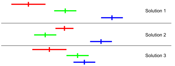
Circular domination is less likely to occur with smaller confidence intervals, i.e. better approximations. The effect of circular domination is that the non-dominated sort algorithm gets stuck because there is no non-dominated front once the circularly dominated solutions are encountered. Because of this reason, this fitness function was not explored further in this text, but the approach described in Section 2.4.2 was used instead.
1In the absence of an algorithm which can provably find the Pareto-optimal set, the term “best effort Pareto-optimal” is here used to denote the set found by a heuristic algorithm designed to converge towards the true Pareto-optimal set.
2A set of Pareto-optimal solutions is by necessity discrete and described only in the points where solutions exist. The term Pareto-front is here used to denote the often continuous space in which all points are Pareto-optimal.